How to Convert Dates to Fiscal Quarters in Google Sheets

This guide will discuss how to convert dates to fiscal quarters in Google Sheets. 

In other words, we will learn how to get the fiscal quarter value from a date value in Google Sheets. This would mean extracting if the given date is from the fiscal year’s Q1, Q2, Q3, or Q4.

Most businesses utilize the fiscal quarters in their financial reports. So it will make the work more efficient if we convert the dates to fiscal quarters in Google Sheets.

But there is not one function in Google Sheets that automatically converts dates to quarters. Instead, we will use the CHOOSE and ROUNDUP functions to do this.

Let’s take, for instance.

Suppose you are making the financial report for the year 2021. It would take too much time to type in what fiscal quarter each date belongs to individually. So you utilize the CHOOSE function to automatically convert inputted dates to the fiscal quarter it belongs to.

Now, you do not have to worry about manually inputting the fiscal quarters. Great! Let’s move on to examine and learn how to write the CHOOSE function and the ROUNDUP function.  

The Anatomy of the CHOOSE Function

So the syntax of the CHOOSE function is as follows:

 =CHOOSE(index, choice1, [choicw2, …])

Let’s examine the formula and understand what each term means:

• = this is to start the function. Every function in Google Sheets begins with the equal sign. 

• CHOOSE() this is our CHOOSE function. CHOOSE is used to select or choose a value from a list of values. Also, this function automatically updates the list of values when you add or remove something from the list. 

• index refers to the numerical value that will decide what choice will be returned. In this case, we will use the MONTH function to get the month value from the date. And the month value will range from 1 to 12, and this will serve as our index. 

• choice1  refers to the value that will be returned if the index value is 1. Additionally, this can be any type of data like a date, formula, number, or text. Also, this is a mandatory argument. 

• choice2 refers to the value that will be returned if the index value is 2. But this is an optional argument. There can be several choices for the CHOOSE function. For instance, we need to get the fiscal quarters. So we will have 12 choices which represent each month.

The Anatomy of the ROUNDUP Function

The way we write, or the syntax, of the ROUNDUP function, is:

 =ROUNDUP(value, [places])

Then, let’s dissect the syntax and learn what each term means:

• = the equal sign is always used to start any function in Google Sheets.

• ROUNDUP() is our ROUNDUP function. This function, from the name, rounds up a number or value. 

• value refers to the number or value that we will round up. 
• places refers to the number of decimal places the value should be rounded up to. Since this is optional, the default decimal place is zero if not specified.  

After learning about the anatomy of the CHOOSE and ROUNDUP functions, let’s dive into a real example where we used these functions to convert dates to fiscal quarters in Google Sheets. 

A Real Example of Converting Dates to Fiscal Quarters in Google Sheets

First, examine the sample spreadsheet below where you need to convert the dates to fiscal quarters. For instance, you are making a financial report on the company sales during the first half of 2022.

We will be doing two ways to convert the dates in column C to fiscal quarters. So we will use the CHOOSE function. First, we get the month value from the range of 1 to 12 using the MONTH function, which will serve us our index. Then, we will input our choices. 

Since the fiscal quarters refer to three months in a year,  our choices are 1,1,1,2,2,2,3,3,3,4,4,4. Finally, the CHOOSE function will return a value from the choices depending on the index. 

For instance, the date 1/15/2022 has an index of 1 because it’s the month of January. So we will get the first value from the choices, which is 1. Thus, the date 1/15/2022 belongs to Quarter 1, or Q1 of the fiscal year.

The second method we will be using is the ROUNDUP function. In this case, we simply divide the month value by 3 since each fiscal quarter has three months. Then, the ROUNDUP function will round up the results to the nearest whole number or integer. 

Furthermore, we will use the CONCATENATE function to return the result as Q1, Q2, Q3, and Q4 instead of just 1, 2, 3, and 4. This function allows us to combine text from different cells.

Finally, this is the final output of converting dates to fiscal quarters in Google Sheets.

You can make your own copy of the spreadsheet above using the link attached below. 

Now that you’ve seen a real example of converting dates to fiscal quarters, it’s time to learn the step-by-step process to apply to your work. 

How to Convert Dates To Fiscal Quarters in Google Sheets

This section will discuss the steps in how to convert dates to fiscal quarters in Google Sheets using two methods.

1. First, we will use the CHOOSE function to convert the dates to fiscal quarters. Type in ‘=’ to start the function and type in the name. Next, type in ‘MONTH’ to start the MONTH function.

Then, select the date we want to convert. In this case, we will select C2. Lastly, type in the choices which are ‘1,1,1,2,2,2,3,3,3,4,4,4’. Press enter to return results.

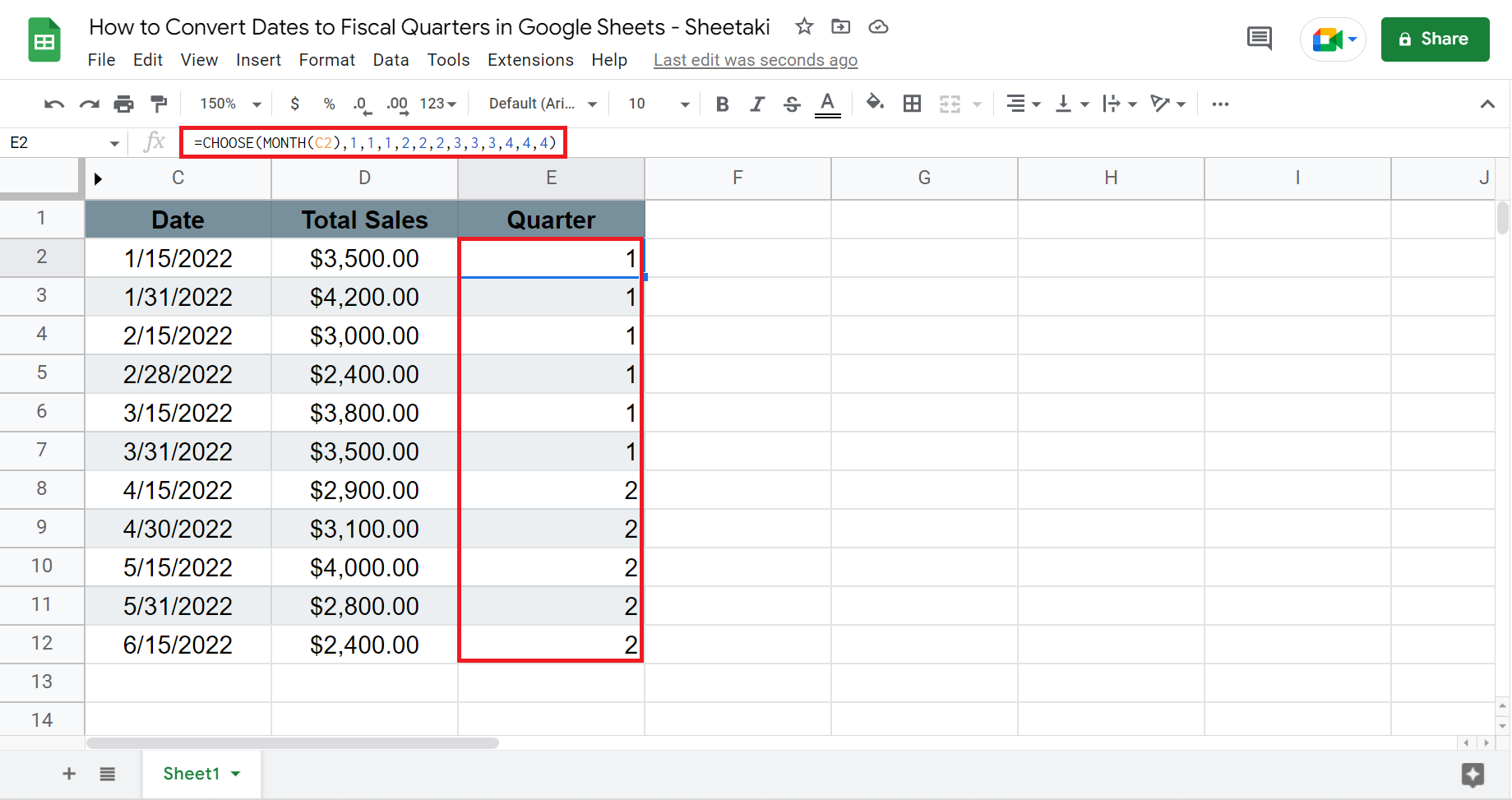
Then, the formula would be =CHOOSE(MONTH(C2),1,1,1,2,2,2,3,3,3,4,4,4).

2. Drag or copy the same formula to the rest of the rows. Otherwise, a suggested auto-fill may appear, and we can simply click check to apply the formula.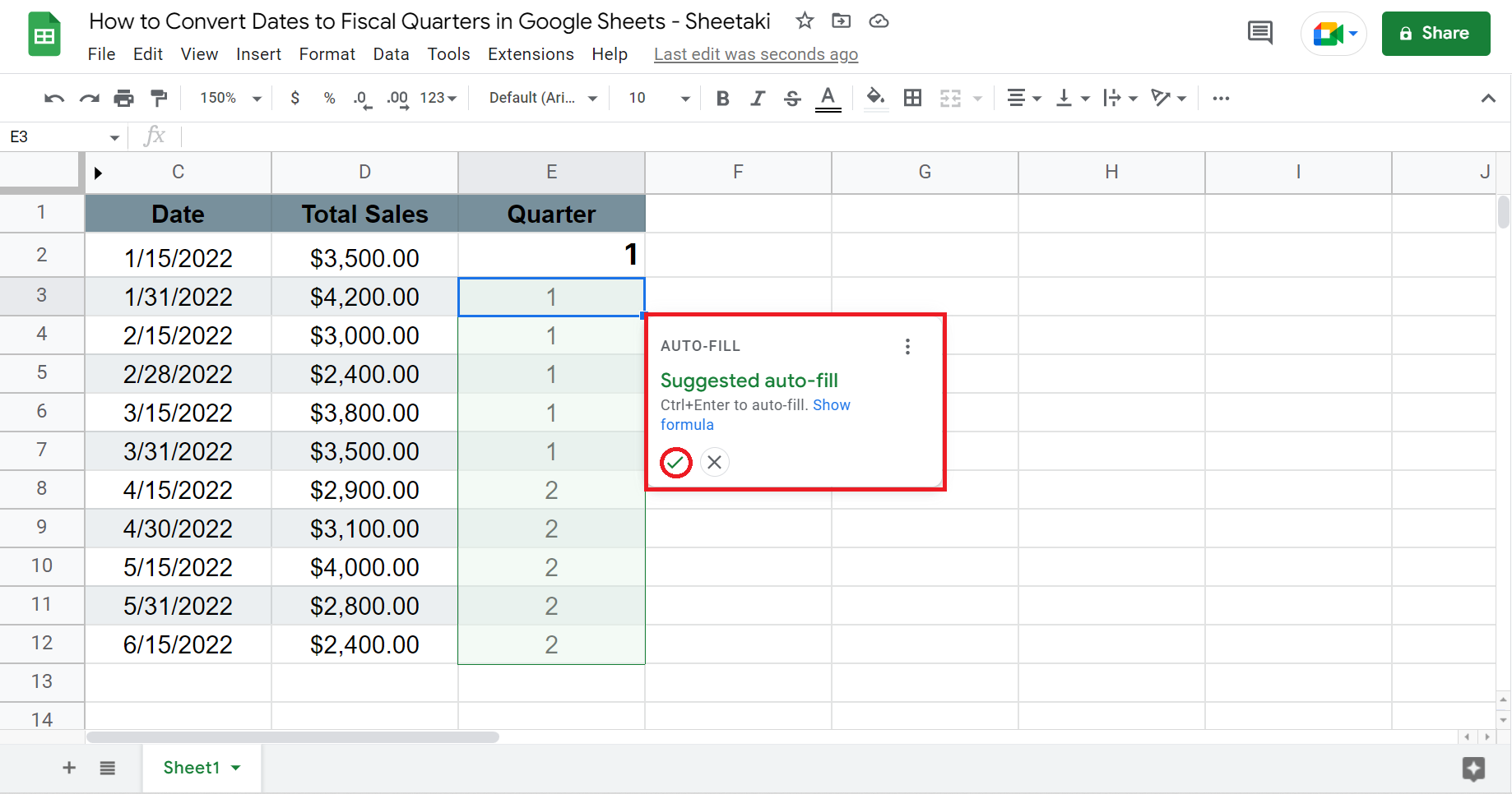

3. The second method uses the ROUNDUP function. Type in ‘=’ and ‘ROUNDUP’. Then, type in ‘MONTH’ and select the date we will convert. Again, this is C2. Next, type in ‘/’ to divide it by 3 and type ‘0’, which is the number of decimal places we want to round up the value.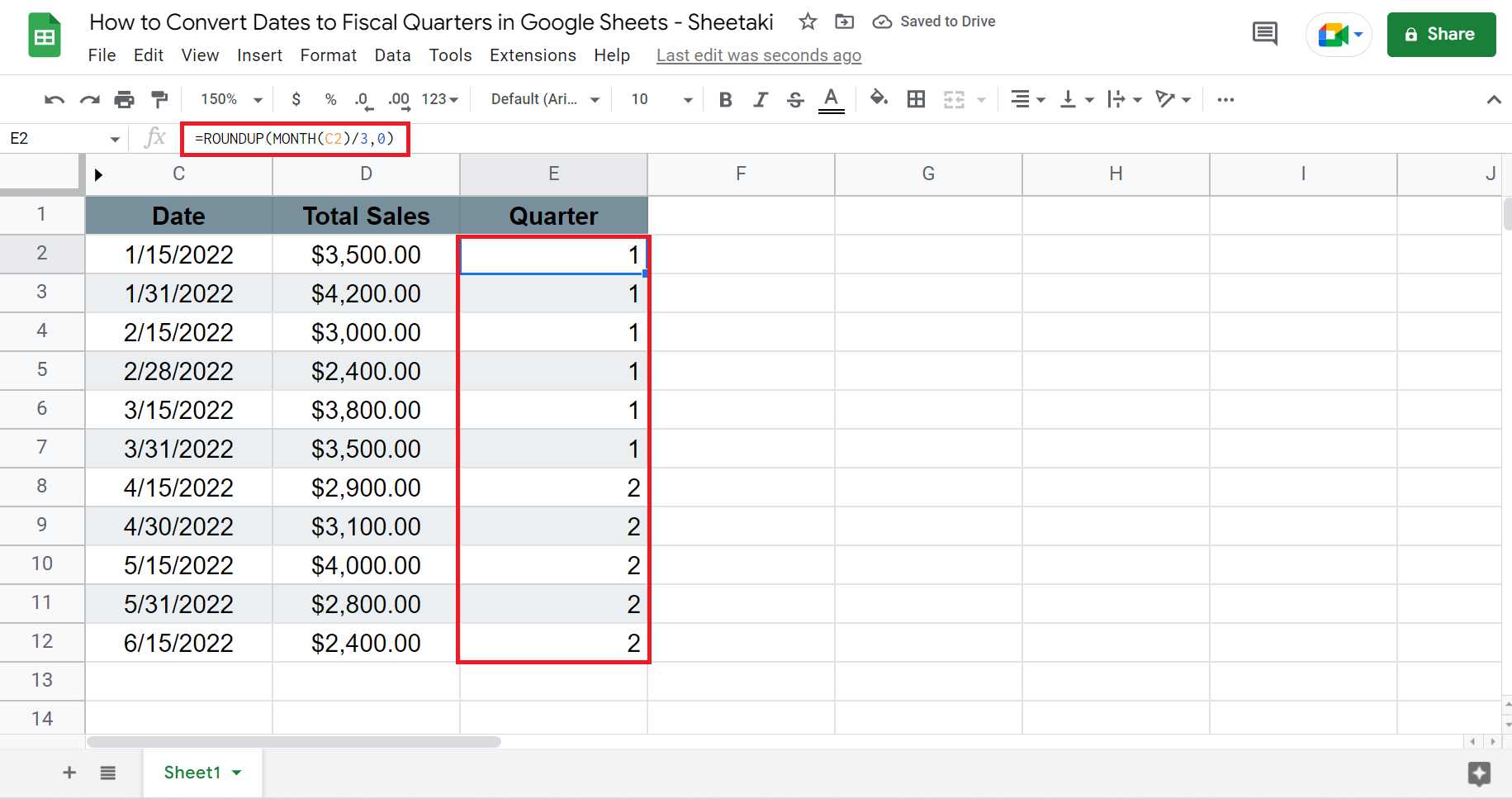

So the entire formula would be =ROUNDUP(MONTH(C2)/3,0) 

4. Again, drag the formula down to apply to the rest of the rows. You can also accept the suggested auto-fill to do the same thing.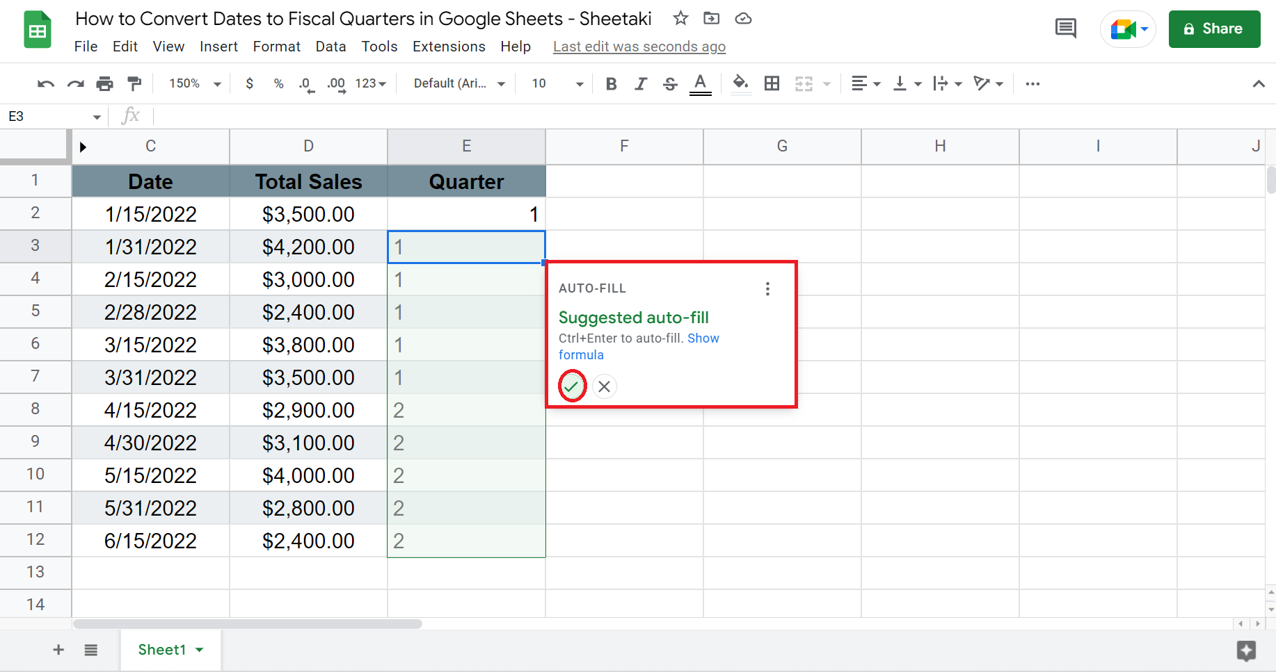

5. If you want the results to return as Q1 or Q2, we can use the CONCATENATE function. Simply add ‘CONCATENATE(“Q”)’ to the ROUNDUP formula. So the formula will be =CONCATENATE(“Q”,ROUNDUP(MONTH(C2)/3,0)). Again, apply the same to the remaining cells in the column.

6. And tada! You have successfully converted the dates to fiscal quarters in Google Sheets.

Finally, you have learned how to convert dates to fiscal quarters in Google Sheets. Surely, this will make your work more efficient, especially when dealing with financial reports or data that require fiscal quarters. 

Are you interested in learning more about what Google Sheets can do? Make sure to subscribe to our newsletter to be the first to know about the latest guides and tutorials from us.

Get emails from us about Google Sheets.

Our goal this year is to create lots of rich, bite-sized tutorials for Google Sheets users like you. If you liked this one, you'll love what we are working on! Readers receive ✨ early access ✨ to new content.

Subscribe