This guide will explain how to highlight same-day duplicates in Google Sheets.
Google Sheets offers multiple methods to find and highlight duplicates in a dataset. To narrow down the results, you may want to restrict it to only count the duplicate entries that fall on the same date.
For example, you have a table of orders with a corresponding product name and date of purchase. You want to highlight all products that have been ordered at least twice on the same day.
In this guide, we will provide a step-by-step tutorial on how to highlight same-day duplicates in Google Sheets.
A Real Example of Highlighting Same-Day Duplicates in Google Sheets
Let’s look into a basic example where we need to highlight same-day duplicates in a dataset.
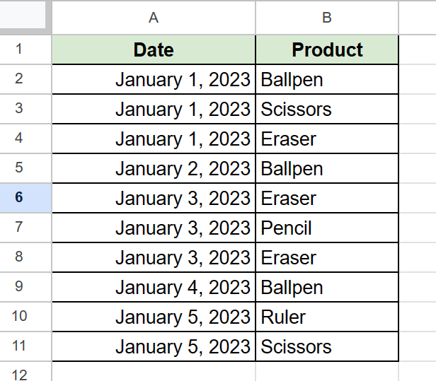
In the example above, we have a dataset that lists orders chronologically by Date. Each order includes exactly one product indicated in the Product field.
We want to highlight cells in column B that are same-day duplicates. For example, we must highlight cells B6 and B8 since they have the same Product value and fall under the same Date.
Before we can highlight same-day duplicates, we must first create a formula that can output all products ordered on a given day.

In the image above, we used the FILTER function to retrieve all products that were ordered on the date indicated in cell A2.
We’ll use the following formula to retrieve all products ordered on January 1, 2023:
=FILTER($B$2:$B,INT($A$2:$A)=INT($A2))
The FILTER function allows users to filter a range based on provided criteria. The first argument indicates the range to filter and the second argument indicates the criteria to use when filtering.
In our formula, we’ve selected the range $B$2:$B since we want to output an array of product names. Our formula uses the criteria INT($A$2:$A)=INT($A2) to compare the values in column A with the date of the current entry (January 1, 2023). The INT function is used to ensure that all date values are converted into an integer before the comparison.

Once we have a FILTER function to obtain all entries under the same date, we can now look for same-day duplicates. We’ll use the COUNTIF function on the FILTER result to find the number of times a specific product appears.
In the image above, we’ve determined that there is only one instance of a ‘Ballpen’ ordered on January 1st, 2023.
We’ll use the following formula to count the number of orders for a ballpen on January 1st, 2023:
=COUNTIF(FILTER($B$2:$B,INT($A$2:$A)=INT($A2)),B2)
Since we want to highlight cells with same-day duplicates, we’ll need to use the Conditional Formatting tool. This feature allows users to format cells a certain way depending on a given criteria.

In the example above, we used the Conditional Formatting tool to highlight all same-day duplicate values in column B.
Using the custom formula option, we’ve added the following formula as a criteria:
=COUNTIF(FILTER($B$2:$B,INT($A$2:$A)=INT($A2)),B2)>1
The COUNTIF function will only return a value greater than 1 if a product is ordered more than once on the same date. Knowing this, we’ve added a “>1” to our formula to ensure that it returns TRUE when a duplicate is found.
You can make a copy of the spreadsheet above using the link attached below.
Head over to the next section to follow our step-by-step tutorial on highlighting same-day duplicates in your spreadsheet.
How to Highlight Same Day Duplicates in Google Sheets
- Select the range of cells that contain the values you want to highlight.
 In the table above, we’ll select the range B2:B11 since we just want to highlight same-day duplicates under the Product field.
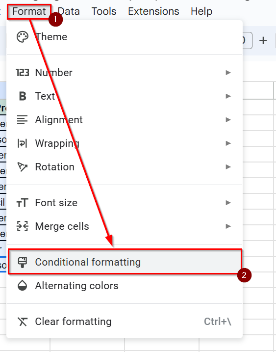
- Next, select the Conditional formatting option under the Format menu.
- A Conditional format rules panel will appear on the right side of your sheet. Ensure you are on the Single color tab then select the Custom formula is option in the dropdown menu under Format rules.

- Apply the formula we’ve described earlier as a formatting rule. Adjust the formatting style to change the way a highlighted cell would appear as. Click on Done to proceed.
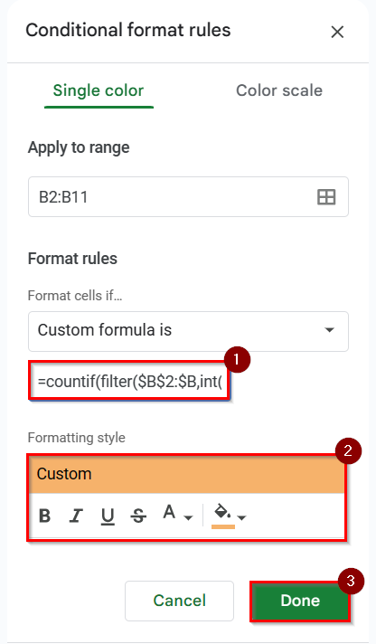 In the above example, we’ve decided to highlight cells by changing their background color to orange.
- Conditional formatting should now highlight all same-day duplicates in the target range.

These are all the steps you need to know to start highlighting same-day duplicates in Google Sheets.
Highlighting same-day duplicates is just one of the many use cases for the conditional formatting tool in Google Sheets. We can also use the Conditional formatting tool to highlight dates that are past a specified deadline.
To learn more advanced spreadsheet techniques, browse our extensive library of Google Sheets resources, tips, and tricks!